Of course! Let's dive deep into numpy.polyfit. It's one of the most fundamental and useful functions for data analysis and curve fitting in Python.

What is numpy.polyfit?

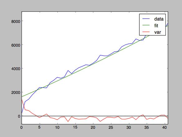
In simple terms, numpy.polyfit is a function that finds the best-fit polynomial for a set of data points.

It uses a mathematical method called least squares regression to find the coefficients of a polynomial that minimizes the sum of the squared differences (the "error") between the actual data points and the points predicted by the polynomial.

The Core Concept: Least Squares Regression

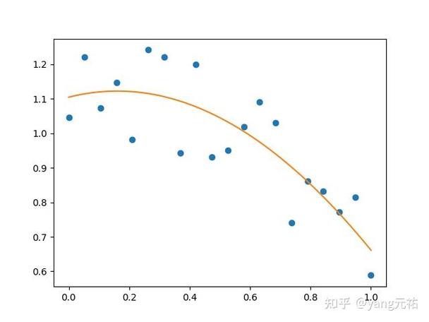
Imagine you have some scattered data points on a graph. You want to draw a smooth curve (a polynomial) that passes as close as possible to all of them. "As close as possible" is defined by minimizing the sum of the vertical distances squared between each data point and the curve.

numpy.polyfit does this for you automatically. It's like drawing the line of best fit, but for any polynomial degree (not just a straight line).

Syntax and Parameters

The function signature is:

numpy.polyfit(x, y, deg, rcond=None, full=False, w=None, cov=False)

Let's break down the most important parameters:

Return Value:

By default, numpy.polyfit returns a 1-D array containing the coefficients of the polynomial, ordered from the highest degree to the lowest.

For example, if you fit a 2nd-degree polynomial (ax² + bx + c), it will return [a, b, c].

Step-by-Step Examples

Let's see it in action with some common scenarios.

Example 1: Fitting a Straight Line (Linear Regression)

This is the most common use case, equivalent to finding the line of best fit.

import numpy as np
import matplotlib.pyplot as plt
# 1. Sample data
x = np.array([0, 1, 2, 3, 4, 5, 6, 7, 8, 9])
y = np.array([1, 3, 2, 5, 7, 8, 8, 9, 10, 12])
# 2. Fit a 1st-degree polynomial (a straight line: y = mx + c)
# The degree 'deg' is 1.
coefficients = np.polyfit(x, y, 1)
print(f"Coefficients (m, c): {coefficients}")
# Expected Output: Coefficients (m, c): [ 1.09090909 -0.30909091]
# The coefficients are [slope, intercept]
m = coefficients[0]
c = coefficients[1]
# 3. Create the polynomial function from the coefficients
# np.poly1d creates a polynomial function from coefficients
poly_function = np.poly1d(coefficients)
# 4. Generate y-values for the line of best fit
y_fit = poly_function(x)
# 5. Plot the results
plt.figure(figsize=(8, 6))
plt.scatter(x, y, color='blue', label='Original Data')
plt.plot(x, y_fit, color='red', linewidth=2, label=f'Fit: y = {m:.2f}x + {c:.2f}')'Linear Fit with numpy.polyfit')
plt.xlabel('X-axis')
plt.ylabel('Y-axis')
plt.legend()
plt.grid(True)
plt.show()

Example 2: Fitting a Quadratic Curve

What if the relationship isn't a straight line? Let's try a 2nd-degree polynomial.

import numpy as np
import matplotlib.pyplot as plt
# 1. Sample data that looks like a parabola
x = np.array([0, 1, 2, 3, 4, 5])
y = np.array([0.5, 2.5, 5.5, 10.5, 17.5, 26.5])
# 2. Fit a 2nd-degree polynomial (ax² + bx + c)
# The degree 'deg' is 2.
coefficients = np.polyfit(x, y, 2)
print(f"Coefficients (a, b, c): {coefficients}")
# Expected Output: Coefficients (a, b, c): [ 1.00000000e+00 -1.11022302e-16  5.00000000e-01]
# Note: The tiny number for 'b' is essentially 0, so the model is y = 1*x² + 0.5
# 3. Create the polynomial function
poly_function = np.poly1d(coefficients)
# 4. Generate y-values for the fitted curve
# Use a finer x-range for a smooth curve
x_fit = np.linspace(0, 5, 100)
y_fit = poly_function(x_fit)
# 5. Plot the results
plt.figure(figsize=(8, 6))
plt.scatter(x, y, color='blue', label='Original Data')
plt.plot(x_fit, y_fit, color='red', linewidth=2, label=f'Fit: {poly_function}')'Quadratic Fit with numpy.polyfit')
plt.xlabel('X-axis')
plt.ylabel('Y-axis')
plt.legend()
plt.grid(True)
plt.show()

Example 3: Handling Noisy Data

Real-world data is often noisy. polyfit is excellent at finding the underlying trend.

import numpy as np
import matplotlib.pyplot as plt
# 1. Generate noisy data around a quadratic trend
np.random.seed(42) # for reproducible results
x = np.linspace(0, 10, 20)
# True relationship is y = 0.5x² - 2x + 5
y_true = 0.5 * x**2 - 2 * x + 5
# Add some random noise
y_noisy = y_true + np.random.normal(0, 3, size=len(x))
# 2. Fit a 2nd-degree polynomial to the noisy data
coefficients = np.polyfit(x, y_noisy, 2)
poly_function = np.poly1d(coefficients)
print(f"Fitted polynomial: {poly_function}")
# Expected Output: Fitted polynomial:           2
#                 0.5028 x - 1.9613 x + 4.6953
# 3. Plot the results
x_fit = np.linspace(0, 10, 100)
y_fit = poly_function(x_fit)
plt.figure(figsize=(8, 6))
plt.scatter(x, y_noisy, color='blue', label='Noisy Data')
plt.plot(x_fit, y_fit, color='red', linewidth=2, label='Fitted Trend')
plt.plot(x_fit, 0.5 * x_fit**2 - 2 * x_fit + 5, color='green', linestyle='--', label='True Model')'Fitting a Noisy Quadratic')
plt.xlabel('X-axis')
plt.ylabel('Y-axis')
plt.legend()
plt.grid(True)
plt.show()

Important Considerations and Pitfalls

Choosing the Right Degree (deg)

This is both an art and a science.

• Underfitting: If you choose a degree that is too low, the polynomial won't capture the trend of the data.

  • Example: Fitting a straight line (deg=1) to parabolic data.

• Overfitting: If you choose a degree that is too high, the polynomial will fit the noise in the data rather than the underlying trend. It will pass very close to your data points but will have a wild, unrealistic shape between them.

  • Example: Fitting a 10th-degree polynomial to 11 data points will result in a polynomial that passes through every single point, but it's almost useless for prediction.

How to choose? Plot the data first! A visual inspection is the best starting point. You can also use metrics like the coefficient of determination (R²) or cross-validation to compare models of different degrees.

Numerical Instability

For very high-degree polynomials or poorly conditioned data (e.g., x values with