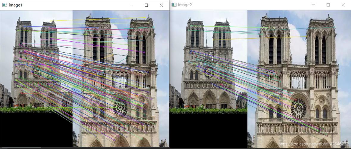
Of course! Let's break down how to combine SIFT (a feature descriptor) with K-Means (a clustering algorithm) in Python. This is a very common and powerful technique in computer vision, most famously used in the Bag-of-Words (BoW) model for image classification.

Here’s a complete guide covering:
- The Big Picture: Why combine SIFT and K-Means?
- Step-by-Step Implementation: A full Python code example.
- Detailed Explanation: What each part of the code does.
- Practical Application: How to use this model to classify images.
The Big Picture: Why SIFT + K-Means?
Think of it like this: how do you compare two documents to see if they are about the same topic? One way is to count the words they use. If they both use the words "market," "stock," and "trade" a lot, they are probably about finance. This is the Bag-of-Words model.
We can apply the exact same idea to images.
- Words in an Image = Visual Words
- Document = Image
- Vocabulary = A set of all possible "visual words"
Here's how SIFT and K-Means fit in:
| Step | Tool | Analogy | What it Does |
|---|---|---|---|
| Find Features | SIFT | Finding keywords in a sentence. | SIFT detects key points (corners, blobs) in an image and calculates a descriptor (a vector of 128 numbers) for each point. This descriptor represents the local appearance around the key point. |
| Build a Vocabulary | K-Means | Grouping all keywords from many books into a standard dictionary. | We take all the SIFT descriptors from all our training images and run K-Means clustering. The cluster centers become our "visual words." We choose k (e.g., 1000) to define the size of our visual vocabulary. |
| Create a Histogram | Counting | Creating a word-frequency histogram for a single book. | For each image, we find its SIFT descriptors and "assign" each one to the nearest visual word (the nearest K-Means cluster center). We then count how many times each visual word appears in the image. This count is a histogram, which becomes the image's feature vector. |
| Compare Images | Distance Metrics | Comparing the word-frequency histograms of two books. | Now that every image is represented by a fixed-length vector (the histogram), we can easily compare them using metrics like L1 distance or Histogram Intersection. This vector can be fed into any standard machine learning classifier (like an SVM) for tasks like image classification. |
Step-by-Step Python Implementation
We'll use popular libraries: OpenCV for SIFT, scikit-learn for K-Means, and matplotlib for visualization.
Prerequisites
First, install the necessary libraries:
pip install opencv-python scikit-learn numpy matplotlib
The Code
This code will:
- Load a few sample images.
- Extract SIFT descriptors from all of them.
- Use K-Means to cluster these descriptors into a "visual vocabulary."
- Show the visual words as images.
- Create a histogram (BoW vector) for one of the images.
import cv2
import numpy as np
from sklearn.cluster import KMeans
import matplotlib.pyplot as plt
from pathlib import Path
# --- 1. Load and Prepare Images ---
# Let's use a few sample images from the scikit-image data module
# or you can provide your own paths.
try:
    from skimage import data
    image1 = cv2.cvtColor(data.astronaut(), cv2.COLOR_RGB2BGR)
    image2 = cv2.cvtColor(data.coffee(), cv2.COLOR_RGB2BGR)
    image3 = cv2.cvtColor(data.horse(), cv2.COLOR_RGB2BGR)
except ImportError:
    print("scikit-image not found. Using placeholder images.")
    # Create some dummy images if scikit-image is not available
    image1 = np.zeros((200, 200, 3), dtype=np.uint8)
    cv2.rectangle(image1, (50, 50), (150, 150), (255, 0, 0), -1)
    image2 = np.zeros((200, 200, 3), dtype=np.uint8)
    cv2.circle(image2, (100, 100), 50, (0, 255, 0), -1)
    image3 = np.zeros((200, 200, 3), dtype=np.uint8)
    cv2.polylines(image3, [np.array([[20,20], [180,20], [100,180]])], True, (0,0,255), 5)
images = [image1, image2, image3]
sift = cv2.SIFT_create()
# --- 2. Extract SIFT Descriptors from ALL Images ---
all_descriptors = []
for img in images:
    # Convert to grayscale as SIFT works on single channel images
    gray = cv2.cvtColor(img, cv2.COLOR_BGR2GRAY)
    # Find keypoints and descriptors
    # We only need descriptors for this task
    _, descriptors = sift.detectAndCompute(gray, None)
    if descriptors is not None:
        all_descriptors.append(descriptors)
# Stack all descriptors into a single NumPy array
# This is our "corpus" of visual words to be clustered
descriptors_stack = np.vstack(all_descriptors)
print(f"Total descriptors extracted: {descriptors_stack.shape[0]}")
print(f"Shape of a single descriptor: {descriptors_stack.shape[1]}")
# --- 3. Build the Visual Vocabulary using K-Means ---
# The number of clusters (k) is the size of our vocabulary
# This is a hyperparameter you can tune
num_clusters = 50
kmeans = KMeans(n_clusters=num_clusters, n_init=10, random_state=42)
print(f"\nRunning K-Means with {num_clusters} clusters on {descriptors_stack.shape[0]} descriptors...")
kmeans.fit(descriptors_stack)
# The cluster centers are our "visual words"
visual_words = kmeans.cluster_centers_
print(f"Shape of visual vocabulary (cluster centers): {visual_words.shape}")
# --- 4. Visualize the Visual Words ---
# Each visual word is a 128-dim vector. We can reshape it to 16x16 and display it.
print("\nVisualizing the visual words (cluster centers)...")
plt.figure(figsize=(10, 5))
for i in range(min(20, num_clusters)): # Show first 20 words
    plt.subplot(4, 5, i + 1)
    word = visual_words[i].reshape(16, 16).astype(np.uint8)
    plt.imshow(word, cmap='gray')
    plt.title(f"Word {i}")
    plt.axis('off')
plt.suptitle("Sample Visual Words (Cluster Centers)")
plt.tight_layout()
plt.show()
# --- 5. Create a Bag-of-Words Histogram for a Single Image ---
# Let's create the BoW vector for the first image
test_image = images[0]
gray_test = cv2.cvtColor(test_image, cv2.COLOR_BGR2GRAY)
_, test_descriptors = sift.detectAndCompute(gray_test, None)
if test_descriptors is not None:
    # Find the nearest visual word for each descriptor in the test image
    # This assigns each descriptor to a cluster (a word)
    word_indices = kmeans.predict(test_descriptors)
    # Create a histogram of word frequencies
    bow_histogram = np.zeros(num_clusters)
    for index in word_indices:
        bow_histogram[index] += 1
    # Normalize the histogram
    bow_histogram = bow_histogram / np.sum(bow_histogram)
    # --- 6. Visualize the Bag-of-Words Histogram ---
    plt.figure(figsize=(10, 5))
    plt.bar(np.arange(num_clusters), bow_histogram)
    plt.title("Bag-of-Words Histogram for the Test Image")
    plt.xlabel("Visual Word Index")
    plt.ylabel("Frequency (Normalized)")
    plt.show()
else:
    print("No descriptors found in the test image.")
Detailed Explanation of the Code
- Load and Prepare Images: We load a few sample images. SIFT works on grayscale images, so we convert them.
- Extract SIFT Descriptors:
- We initialize the SIFT detector:
sift = cv2.SIFT_create(). - We loop through each image, convert it to grayscale, and call
sift.detectAndCompute(). - This function returns two things:
keypoints(the locations of features) anddescriptors(the 128-dim vectors for those features). For the BoW model, we only care about the descriptors. - We collect all descriptors from all images into a list and then stack them into one big NumPy array. This array is our dataset for K-Means.
- We initialize the SIFT detector:
- Build Visual Vocabulary with K-Means:
- We decide on a
num_clusters(e.g., 50, 100, 1000). This is the size of our vocabulary. More clusters can capture more detail but also increases dimensionality and computation time. - We create a
KMeansobject fromscikit-learnand fit it to ourdescriptors_stack. - After fitting,
kmeans.cluster_centers_holds the coordinates of the cluster centers. These centers are our visual words. Each one is a representative "average" patch from all the patches we saw in our training data.
- We decide on a
- Visualize Visual Words: Since a 128-dim vector is hard to look at, we reshape each one to a 16x16 image patch. This gives you an intuitive idea of what your "words" look like. They will often resemble simple patterns like edges, corners, or blobs.
- Create a Bag-of-Words Histogram:
- We take a new, unseen image (
test_image). - We extract its SIFT descriptors.
- We use the already trained
kmeansmodel topredictwhich cluster (visual word) each of our new descriptors belongs to. This gives us a list of word indices. - We create a histogram (a vector of size
num_clusters) and count the occurrences of each word index. - Finally, we normalize the histogram so that the sum of its elements is 1. This makes the representation independent of the image size or the number of features detected.
- We take a new, unseen image (
Practical Application: Image Classification
Now that you know how to create the BoW vector for an image, here's how you'd use it for a real task.
# Conceptual Code for Image Classification
# --- Step A: Prepare Data for ALL Training Images ---
# (This is a simplified version of the code above, but for a whole dataset)
# Assume you have lists: `all_train_images` and `all_train_labels`
# train_bow_vectors = []
# for image in all_train_images:
#     gray = cv2.cvtColor(image, cv2.COLOR_BGR2GRAY)
#     _, descriptors = sift.detectAndCompute(gray, None)
#     if descriptors is not None:
#         word_indices = kmeans.predict(descriptors)
#         bow_histogram = np.zeros(num_clusters)
#         np.add.at(bow_histogram, word_indices, 1) # Efficient counting
#         bow_histogram = bow_histogram / np.sum(bow_histogram)
#         train_bow_vectors.append(bow_histogram)
# train_bow_vectors = np.array(train_bow_vectors)
# --- Step B: Train a Classifier ---
# from sklearn.svm import SVC
# from sklearn.model_selection import train_test_split
# from sklearn.metrics import accuracy_score
# # X: feature vectors, y: labels
# X_train, X_test, y_train, y_test = train_test_split(
#     train_bow_vectors, all_train_labels, test_size=0.2, random_state=42
# )
# classifier = SVC(kernel='linear', C=1.0)
# print("Training SVM classifier...")
# classifier.fit(X_train, y_train)
# # --- Step C: Evaluate the Classifier ---
# # You would repeat Step A for your test images to get test_bow_vectors
# # predictions = classifier.predict(X_test)
# # accuracy = accuracy_score(y_test, predictions)
# # print(f"Classification Accuracy: {accuracy * 100:.2f}%")
This workflow is the foundation for many classical computer vision tasks before the deep learning era. While deep learning (like CNNs) has largely surpassed it for classification, the BoW model is still an excellent concept to understand and is used in applications like image retrieval and visual search.

