Here is a complete guide to implementing Naive Bayes in Python.

There are two ways to do this:

1. Using Scikit-Learn: The industry-standard way (easy, fast, optimized).
2. From Scratch: The educational way (to understand the math).

The Practical Approach (Scikit-Learn)

For real-world projects, you should use scikit-learn. The most common version is Multinomial Naive Bayes, which is famous for text classification (like Spam vs. Ham).

Here is a full example using the classic "20 Newsgroups" dataset to classify text topics.

import pandas as pd
from sklearn.feature_extraction.text import CountVectorizer
from sklearn.model_selection import train_test_split
from sklearn.naive_bayes import MultinomialNB
from sklearn.metrics import accuracy_score, classification_report
# 1. Create a dummy dataset (Text, Label)
data = {
    'text': [
        "Free money now!!!", 
        "Hi Bob, how about a game of golf tomorrow?",
        "URGENT! Your bank account is compromised.",
        "Meeting reminder: Project sync at 10 AM.",
        "Win a brand new car! Click here.",
        "Can we reschedule dinner to next week?",
        "Limited time offer! Buy one get one free.",
        "Don't forget to bring the snacks for the party."
    ],
    'label': ['spam', 'ham', 'spam', 'ham', 'spam', 'ham', 'spam', 'ham']
}
df = pd.DataFrame(data)
# 2. Convert text to numbers (Bag of Words)
# Naive Bayes cannot read text; it needs frequency counts.
vectorizer = CountVectorizer(stop_words='english')
X = vectorizer.fit_transform(df['text'])
y = df['label']
# 3. Split data
X_train, X_test, y_train, y_test = train_test_split(X, y, test_size=0.3, random_state=42)
# 4. Initialize and Train the Model
model = MultinomialNB()
model.fit(X_train, y_train)
# 5. Make Predictions
y_pred = model.predict(X_test)
# 6. Evaluate
print(f"Accuracy: {accuracy_score(y_test, y_pred)}")
print("\nClassification Report:\n", classification_report(y_test, y_pred))
# Test on a new sentence
new_sentence = ["Congratulation! You won the lottery."]
new_sentence_vectorized = vectorizer.transform(new_sentence)
prediction = model.predict(new_sentence_vectorized)
print(f"\nPrediction for '{new_sentence[0]}': {prediction[0]}")

Choosing the Right Naive Bayes

Scikit-learn offers three main types. You must choose based on your data distribution:

1. MultinomialNB: Best for Text (Word counts, TF-IDF).
   • Example: Spam filtering, Topic categorization.
2. GaussianNB: Best for Continuous Features (assuming a normal distribution).
   • Example: Iris flower classification (petal length/width).
3. BernoulliNB: Best for Binary Features (presence/absence).
   • Example: Checking if specific words exist in a document (yes/no).

Example: Gaussian Naive Bayes (Continuous Data)

from sklearn.datasets import load_iris
from sklearn.naive_bayes import GaussianNB
from sklearn.model_selection import train_test_split
# Load data
iris = load_iris()
X, y = iris.data, iris.target
# Split
X_train, X_test, y_train, y_test = train_test_split(X, y, test_size=0.3)
# Model
gnb = GaussianNB()
gnb.fit(X_train, y_train)
# Predict
print("Predictions:", gnb.predict(X_test))

The "From Scratch" Approach (Educational)

To understand how it works, here is a simplified implementation using only Python standard libraries.

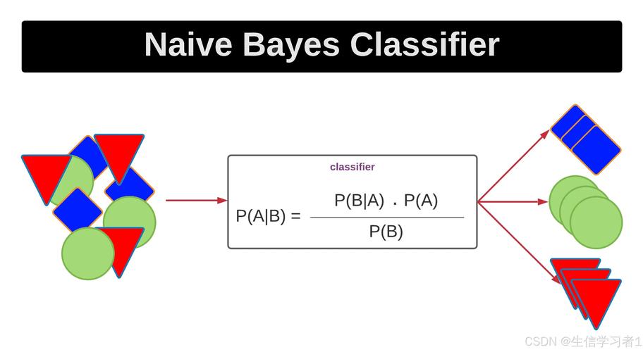
Naive Bayes calculates: $P(Class | Features) \propto P(Class) \times P(Feature | Class)$

import numpy as np
class NaiveBayesScratch:
    def fit(self, X, y):
        n_samples, n_features = X.shape
        self._classes = np.unique(y)
        n_classes = len(self._classes)
        # Calculate mean, var, and prior for each class
        self._mean = np.zeros((n_classes, n_features), dtype=np.float64)
        self._var = np.zeros((n_classes, n_features), dtype=np.float64)
        self._priors = np.zeros(n_classes, dtype=np.float64)
        for idx, c in enumerate(self._classes):
            X_c = X[y == c]
            self._mean[idx, :] = X_c.mean(axis=0)
            self._var[idx, :] = X_c.var(axis=0)
            self._priors[idx] = X_c.shape[0] / float(n_samples)
    def predict(self, X):
        y_pred = [self._predict(x) for x in X]
        return np.array(y_pred)
    def _predict(self, x):
        posteriors = []
        # Calculate posterior probability for each class
        for idx, c in enumerate(self._classes):
            prior = np.log(self._priors[idx])
            posterior = np.sum(np.log(self._pdf(idx, x)))
            posterior = prior + posterior
            posteriors.append(posterior)
        # Return class with highest posterior
        return self._classes[np.argmax(posteriors)]
    def _pdf(self, class_idx, x):
        # Probability Density Function (Gaussian)
        mean = self._mean[class_idx]
        var = self._var[class_idx]
        numerator = np.exp(-((x - mean) ** 2) / (2 * var))
        denominator = np.sqrt(2 * np.pi * var)
        return numerator / denominator
# Testing the scratch model
from sklearn.datasets import make_classification
X, y = make_classification(n_samples=100, n_features=2, n_classes=2, n_redundant=0, random_state=42)
model = NaiveBayesScratch()
model.fit(X, y)
predictions = model.predict(X)
print(f"Accuracy from scratch: {np.mean(predictions == y)}")

Summary of Pros and Cons

Pros:

• Extremely Fast: Training is almost instantaneous.
• Works on Small Data: Doesn't need massive datasets to work well.
• Good for Text: Handles high-dimensional data (like thousands of words) better than many complex algorithms.

Cons:

• The "Naive" Assumption: It assumes features are independent (e.g., the word "Bank" appearing is unrelated to the word "Money" appearing). In reality, this is rarely true, but the algorithm works anyway.
• Zero Frequency: If a word appears in the test set but not the training set, the probability becomes zero. (Scikit-learn handles this automatically using a parameter called alpha for smoothing).