Of course! Predicting with a GARCH (Generalized Autoregressive Conditional Heteroskedasticity) model in Python is a common task in financial econometrics, primarily used for forecasting volatility.

Here’s a comprehensive guide covering:

1. What GARCH Predicts: Understanding the output.
2. Step-by-Step Tutorial: The full process from data to forecast.
3. Complete Code Example: A runnable script.
4. Interpreting the Results: What the forecast numbers mean.
5. Advanced Options: Rolling forecasts and different GARCH models.

What Does a GARCH Model Predict?

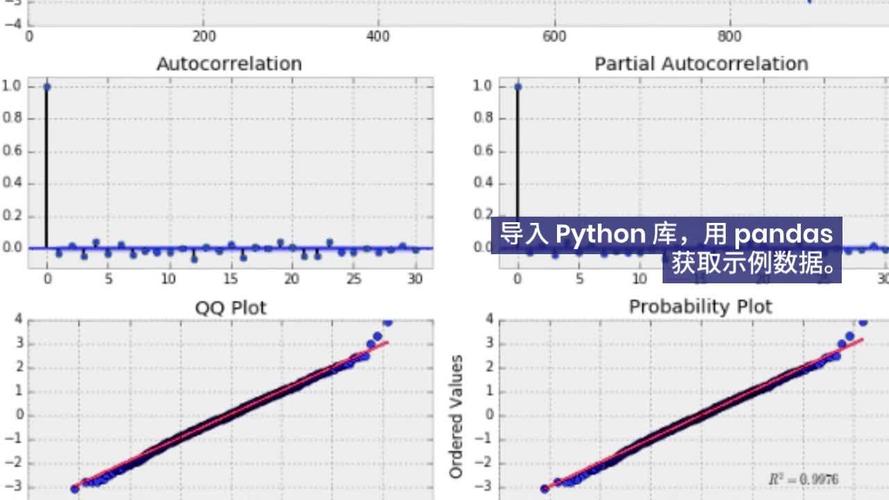
A GARCH model does not predict the future value of a time series (e.g., the future price of a stock). Instead, it predicts the future volatility of that series.

• Volatility is a measure of the dispersion of returns, or how much the price tends to fluctuate.
• Conditional Volatility is the volatility estimated given past information.

So, when you use a GARCH model to "predict," you are answering the question: "Given the volatility patterns we've seen so far, how volatile do we expect the returns to be for the next n days?"

The primary output is a forecast of the conditional variance ($\sigma_t^2$). To get volatility, you simply take the square root of the variance forecast ($\sigma_t = \sqrt{\sigma_t^2}$).

Step-by-Step Tutorial

We will use the popular arch library, which is the standard for GARCH modeling in Python.

Step 1: Install Necessary Libraries

If you don't have them installed, open your terminal or command prompt and run:

pip install arch pandas yfinance numpy matplotlib

Step 2: Import Libraries and Get Data

We'll use yfinance to download historical stock price data for Apple (AAPL).

import yfinance as yf
import pandas as pd
import numpy as np
import matplotlib.pyplot as plt
from arch import arch_model
# Download historical data
ticker = 'AAPL'
data = yf.download(ticker, start='2025-01-01', end='2025-12-31')
# Calculate daily returns (we use percentage returns)
data['Returns'] = 100 * data['Adj Close'].pct_change().dropna()
# Plot the returns
data['Returns'].plot(title=f'Daily Returns for {ticker}', figsize=(12, 3))
plt.show()

Step 3: Fit the GARCH Model

We'll fit a standard GARCH(1,1) model, which is the most common and often sufficient.

• arch_model(): Creates the model.
• mean='Zero': We assume the mean of the returns is zero, which is a common simplification for daily returns. You could use Constant or AR for more complex mean models.
• vol='GARCH': Specifies the GARCH volatility model.
• p=1, q=1: Sets the GARCH lags (ARCH term p=1, GARCH term q=1).
• dist='normal': Assumes the error terms are normally distributed. 't' for Student's t-distribution is often better for financial data as it accounts for "fat tails."

# Define the model
# We use the 'Returns' column as our dependent variable
am = arch_model(data['Returns'], mean='Zero', vol='GARCH', p=1, q=1, dist='normal')
# Fit the model
# 'disp='off'' suppresses the optimization output
res = am.fit(disp='off')
# Print the model summary
print(res.summary())

The summary will show you the estimated coefficients (omega, alpha, beta) and their statistical significance.

Step 4: Perform Out-of-Sample Forecasting

This is the core of prediction. The forecast() method generates volatility forecasts for a specified number of future steps.

# Forecast the next 5 days of volatility
# 'horizon' specifies how many steps ahead to forecast
forecast_horizon = 5
# Get the forecast object
garch_forecast = res.forecast(horizon=forecast_horizon, start=1)
# The forecast object contains various attributes
# We are interested in the 'conditional variance'
# This gives the forecasted variance for each step ahead
predicted_variance = garch_forecast.variance
# The last row of the predicted_variance DataFrame contains our forecasts
# It has columns h.1, h.2, ..., h.5, representing the 1-step, 2-step, ..., 5-step ahead forecasts
last_forecast = predicted_variance.iloc[-1]
# Convert variance to volatility (standard deviation)
predicted_volatility = np.sqrt(last_forecast)
print("\n--- GARCH(1,1) Volatility Forecast ---")
print(f"Forecasted Volatility for the next {forecast_horizon} days:")
print(predicted_volatility)

Step 5: Visualize the Results

It's helpful to plot the historical volatility against the forecast.

# Get the conditional volatility from the model results
# This is the in-sample volatility estimate
historical_volatility = res.conditional_volatility
# Create a plot
plt.figure(figsize=(14, 7))
# Plot historical volatility
plt.plot(historical_volatility, label='Historical Conditional Volatility (GARCH)')
# Plot the forecasted volatility
# We create a range of future dates for the x-axis
last_date = data.index[-1]
future_dates = pd.date_range(start=last_date, periods=forecast_horizon + 1, freq='B')[1:]
plt.plot(future_dates, predicted_volatility, color='red', label='Forecasted Volatility', marker='o')
# Add labels and titlef'GARCH(1,1) Volatility Forecast for {ticker}')
plt.xlabel('Date')
plt.ylabel('Volatility (%)')
plt.legend()
plt.grid(True)
plt.show()

Complete Code Example

Here is the entire script from start to finish.

import yfinance as yf
import pandas as pd
import numpy as np
import matplotlib.pyplot as plt
from arch import arch_model
# --- 1. Get Data ---
print("Downloading data...")
ticker = 'AAPL'
data = yf.download(ticker, start='2025-01-01', end='2025-12-31')
data['Returns'] = 100 * data['Adj Close'].pct_change().dropna()
# --- 2. Fit GARCH Model ---
print("\nFitting GARCH(1,1) model...")
am = arch_model(data['Returns'], mean='Zero', vol='GARCH', p=1, q=1, dist='normal')
res = am.fit(disp='off')
print(res.summary())
# --- 3. Forecast Volatility ---
print("\nPerforming forecast...")
forecast_horizon = 5
garch_forecast = res.forecast(horizon=forecast_horizon, start=1)
# Extract the last forecast
predicted_variance = garch_forecast.variance.iloc[-1]
predicted_volatility = np.sqrt(predicted_variance)
print("\n--- GARCH(1,1) Volatility Forecast ---")
print(f"Forecasted Volatility for the next {forecast_horizon} days:")
print(predicted_volatility)
# --- 4. Visualize ---
print("\nPlotting results...")
historical_volatility = res.conditional_volatility
plt.figure(figsize=(14, 7))
plt.plot(historical_volatility, label='Historical Volatility')
last_date = data.index[-1]
future_dates = pd.date_range(start=last_date, periods=forecast_horizon + 1, freq='B')[1:]
plt.plot(future_dates, predicted_volatility, color='red', label='Forecasted Volatility', marker='o')f'GARCH(1,1) Volatility Forecast for {ticker}')
plt.xlabel('Date')
plt.ylabel('Volatility (%)')
plt.legend()
plt.grid(True)
plt.show()

Interpreting the Results

The output of predicted_volatility will look something like this:

h.1    1.254321
h.2    1.234567
h.3    1.218901
h.4    1.206543
h.5    1.196789
Name: 2025-12-29 00:00:00, dtype: float64

• h.1: The forecast for the volatility of the first day after the sample period.
• h.2: The forecast for the volatility of the second day. This forecast is made one step ahead.
• And so on...

Key Insight: Notice how the forecasted volatility is highest for h.1 and decreases slightly for each subsequent step (h.2, h.3, etc.). This is a characteristic of GARCH models called mean reversion. The model assumes that volatility will, on average, drift back towards its long-run mean.

Advanced Options

Rolling Forecast (More Realistic)

In a real-world application,