Of course! Calculating Value at Risk (VaR) is a fundamental task in financial risk management. Python is an excellent tool for this due to its powerful libraries for data analysis and numerical computation.

This guide will walk you through:
- What is VaR? A quick conceptual overview.
- Three Main Methods for calculating VaR.
- Complete Python Code Examples for each method.
- A Complete Script that you can run and adapt.
- Advantages and Disadvantages of each approach.
What is Value at Risk (VaR)?
Value at Risk (VaR) is a statistical measure that quantifies the potential loss in value of a portfolio over a specific time period for a given confidence level.
In simpler terms, it answers the question: "What is my maximum expected loss with X% confidence over the next N days?"
- Portfolio: A collection of assets (stocks, bonds, etc.).
- Time Horizon (N): The period you're looking at (e.g., 1 day, 10 days).
- Confidence Level (X%): The probability that the loss will not exceed the VaR. (e.g., 95%, 99%).
Example:

A portfolio has a 1-day 95% VaR of $1 million.
- Interpretation: There is a 95% probability that the portfolio will not lose more than $1 million in the next day.
- Equivalently: There is a 5% chance that the portfolio will lose more than $1 million in the next day. This 5% is the "tail risk."
Three Main Methods for Calculating VaR
There are three primary methods to calculate VaR, each with its own assumptions and strengths.
| Method | Description | Pros | Cons |
|---|---|---|---|
| Historical Simulation | Uses actual historical returns to simulate future returns. No assumptions about the distribution of returns. | - Simple to implement. - Captures "fat tails" and non-normal market behavior. - Intuitive. |
- Assumes the past is a perfect predictor of the future. - VaR can be sensitive to the chosen historical period. |
| Parametric (Variance-Covariance) | Assumes returns are normally distributed. It uses the mean (expected return) and standard deviation (volatility) of the portfolio. | - Computationally very fast. - Provides a smooth, continuous VaR estimate. |
- The main weakness: returns are not normally distributed. They often have "fat tails," meaning extreme events happen more often than a normal distribution predicts. |
| Monte Carlo Simulation | Generates thousands of random potential future scenarios for asset returns based on a specified distribution (e.g., geometric Brownian motion). | - Very flexible. You can model complex instruments and non-normal distributions. - Can capture a wide range of risks. |
- Computationally intensive. - Results depend heavily on the assumptions of the model you choose to generate the scenarios. |
Python Code Examples
First, make sure you have the necessary libraries installed:
pip install numpy pandas yfinance matplotlib scipy
We'll use yfinance to download historical stock data.

Setup: Get Portfolio Data
Let's assume we have a simple portfolio of 3 stocks: Apple (AAPL), Microsoft (MSFT), and Google (GOOG). We'll get their historical prices and calculate daily returns.
import yfinance as yf
import numpy as np
import pandas as pd
import matplotlib.pyplot as plt
from scipy.stats import norm
# --- 1. GET DATA ---
# Define the stocks and the date range
tickers = ['AAPL', 'MSFT', 'GOOG']
start_date = '2025-01-01'
end_date = '2025-12-31'
# Download adjusted close prices
data = yf.download(tickers, start=start_date, end=end_date)['Adj Close']
# Calculate daily returns
returns = data.pct_change().dropna()
# Define portfolio weights (e.g., equal weight)
weights = np.array([0.33, 0.33, 0.34])
portfolio_returns = (returns * weights).sum(axis=1)
print("Portfolio Daily Returns Head:")
print(portfolio_returns.head())
Method 1: Historical Simulation VaR
This is the most straightforward method. We simply sort the historical portfolio returns and find the loss at the desired percentile.
def calculate_historical_var(returns, confidence_level=0.95):
    """
    Calculates VaR using the Historical Simulation method.
    Args:
        returns (pd.Series): A series of historical portfolio returns.
        confidence_level (float): The confidence level (e.g., 0.95 for 95%).
    Returns:
        float: The calculated VaR.
    """
    # The VaR is the negative of the percentile of the returns
    # We use (1 - confidence_level) because we are interested in the left tail (losses)
    var = -np.percentile(returns, (1 - confidence_level) * 100)
    return var
# --- Calculate Historical VaR ---
historical_var_95 = calculate_historical_var(portfolio_returns, 0.95)
historical_var_99 = calculate_historical_var(portfolio_returns, 0.99)
print(f"\n--- Historical Simulation VaR ---")
print(f"1-Day 95% VaR: ${historical_var_95:.4f}")
print(f"1-Day 99% VaR: ${historical_var_99:.4f}")
Method 2: Parametric (Variance-Covariance) VaR
This method assumes returns are normally distributed. We need the portfolio's expected return (mean) and standard deviation (volatility).
def calculate_parametric_var(returns, confidence_level=0.95):
    """
    Calculates VaR using the Parametric (Variance-Covariance) method.
    Args:
        returns (pd.Series): A series of historical portfolio returns.
        confidence_level (float): The confidence level.
    Returns:
        float: The calculated VaR.
    """
    # Calculate the portfolio's mean and standard deviation
    mean_return = returns.mean()
    std_dev = returns.std()
    # For VaR, we are typically interested in the short term, so we can assume mean_return is ~0
    # We use the Z-score from the standard normal distribution
    z_score = norm.ppf(1 - confidence_level)
    var = -(mean_return + z_score * std_dev)
    return var
# --- Calculate Parametric VaR ---
parametric_var_95 = calculate_parametric_var(portfolio_returns, 0.95)
parametric_var_99 = calculate_parametric_var(portfolio_returns, 0.99)
print(f"\n--- Parametric VaR ---")
print(f"1-Day 95% VaR: ${parametric_var_95:.4f}")
print(f"1-Day 99% VaR: ${parametric_var_99:.4f}")
Method 3: Monte Carlo Simulation VaR
This method is more complex. We generate random future returns based on a statistical model (usually a Geometric Brownian Motion) and then find the VaR from this simulated distribution.
def calculate_monte_carlo_var(returns, confidence_level=0.95, n_simulations=10000, time_horizon=1):
    """
    Calculates VaR using the Monte Carlo Simulation method.
    Args:
        returns (pd.Series): A series of historical portfolio returns.
        confidence_level (float): The confidence level.
        n_simulations (int): Number of simulations to run.
        time_horizon (int): The time horizon for the VaR (e.g., 1 for 1 day).
    Returns:
        float: The calculated VaR.
    """
    # Calculate drift (mu) and volatility (sigma) from historical data
    mu = returns.mean()
    sigma = returns.std()
    # Generate random numbers from a normal distribution
    random_shocks = np.random.standard_normal(n_simulations)
    # Calculate the simulated returns for the time horizon
    simulated_returns = (mu - 0.5 * sigma**2) * time_horizon + sigma * np.sqrt(time_horizon) * random_shocks
    # The VaR is the negative of the percentile of the simulated returns
    var = -np.percentile(simulated_returns, (1 - confidence_level) * 100)
    return var
# --- Calculate Monte Carlo VaR ---
monte_carlo_var_95 = calculate_monte_carlo_var(portfolio_returns, 0.95)
monte_carlo_var_99 = calculate_monte_carlo_var(portfolio_returns, 0.99)
print(f"\n--- Monte Carlo Simulation VaR ---")
print(f"1-Day 95% VaR: ${monte_carlo_var_95:.4f}")
print(f"1-Day 99% VaR: ${monte_carlo_var_99:.4f}")
Complete, Runnable Script
Here is a full script that combines all the steps and visualizes the results.
import yfinance as yf
import numpy as np
import pandas as pd
import matplotlib.pyplot as plt
from scipy.stats import norm
# --- 1. SETUP: GET DATA ---
def get_portfolio_data(tickers, start_date, end_date):
    """Downloads stock data and calculates portfolio returns."""
    data = yf.download(tickers, start=start_date, end=end_date)['Adj Close']
    returns = data.pct_change().dropna()
    return returns
# --- 2. VaR CALCULATION FUNCTIONS ---
def historical_var(returns, confidence_level):
    return -np.percentile(returns, (1 - confidence_level) * 100)
def parametric_var(returns, confidence_level):
    mean_return = returns.mean()
    std_dev = returns.std()
    z_score = norm.ppf(1 - confidence_level)
    return -(mean_return + z_score * std_dev)
def monte_carlo_var(returns, confidence_level, n_sims=10000):
    mu = returns.mean()
    sigma = returns.std()
    random_shocks = np.random.standard_normal(n_sims)
    simulated_returns = (mu - 0.5 * sigma**2) + sigma * random_shocks
    return -np.percentile(simulated_returns, (1 - confidence_level) * 100)
# --- 3. MAIN EXECUTION ---
if __name__ == "__main__":
    # Define portfolio and time period
    TICKERS = ['AAPL', 'MSFT', 'GOOG']
    START_DATE = '2025-01-01'
    END_DATE = '2025-12-31'
    CONFIDENCE_LEVEL = 0.95
    # Get data
    returns = get_portfolio_data(TICKERS, START_DATE, END_DATE)
    # Use equal weights for simplicity
    portfolio_returns = (returns * np.array([1/len(TICKERS)] * len(TICKERS))).sum(axis=1)
    # Calculate VaR for all methods
    hist_var = historical_var(portfolio_returns, CONFIDENCE_LEVEL)
    para_var = parametric_var(portfolio_returns, CONFIDENCE_LEVEL)
    mc_var = monte_carlo_var(portfolio_returns, CONFIDENCE_LEVEL)
    # --- 4. DISPLAY RESULTS ---
    print(f"--- 1-Day {CONFIDENCE_LEVEL*100:.0f}% VaR for Portfolio ---")
    print(f"Historical Simulation VaR: ${hist_var:.4f}")
    print(f"Parametric (Normal) VaR:   ${para_var:.4f}")
    print(f"Monte Carlo Simulation VaR: ${mc_var:.4f}\n")
    # --- 5. VISUALIZATION ---
    plt.figure(figsize=(12, 6))
    plt.hist(portfolio_returns, bins=100, density=True, alpha=0.75, label='Historical Returns Distribution')
    # Plot VaR lines
    plt.axvline(-hist_var, color='r', linestyle='--', linewidth=2, label=f'Historical VaR (${hist_var:.4f})')
    plt.axvline(-para_var, color='g', linestyle='--', linewidth=2, label=f'Parametric VaR (${para_var:.4f})')
    plt.axvline(-mc_var, color='b', linestyle='--', linewidth=2, label=f'Monte Carlo VaR (${mc_var:.4f})')
    plt.title(f'Portfolio Returns Distribution and {CONFIDENCE_LEVEL*100:.0f}% VaR')
    plt.xlabel('Daily Return')
    plt.ylabel('Density')
    plt.legend()
    plt.grid(True)
    plt.show()
Important Considerations and Caveats
- VaR is Not a "Maximum Loss": VaR does not tell you the maximum you can lose. It only tells you the loss you will exceed with a certain probability (e.g., 5% of the time). The actual loss in those 5% scenarios could be much, much larger. This is where Expected Shortfall (ES) or Conditional VaR (CVaR) comes in, which measures the average loss given that the loss has exceeded the VaR.
- Model Risk: All VaR models are based on assumptions. If your assumptions are wrong (e.g., assuming normality when the market is crashing), your VaR estimate will be wrong.
- VaR Horizons: The examples above are for a 1-day horizon. To scale VaR to a longer horizon (e.g., 10 days), you typically multiply the 1-day VaR by the square root of the number of days (assuming i.i.d. returns):
10_day_var = 1_day_var * sqrt(10). This is known as the "square root of time rule."