Of course! Here is a comprehensive guide to building an ARIMA model in Python, broken down into conceptual explanations, a step-by-step tutorial with code, and advanced considerations.

What is an ARIMA Model?

ARIMA stands for AutoRegressive Integrated Moving Average. It's a powerful and popular statistical model used for time series forecasting.

The model is defined by three key components:

1. AR (AutoRegressive): This part uses the relationship between an observation and a number of lagged observations (previous time steps). For example, it's like saying today's stock price is dependent on the prices of the last few days.

   • p: The number of lag observations included in the model (the "lag order").

2. I (Integrated): This part involves differencing the raw observations to make the time series stationary. A stationary time series has statistical properties (mean, variance, autocorrelation) that do not change over time. Most time series data (like stock prices or sales) are non-stationary.

   • d: The number of times the raw observations are differenced (the "degree of differencing").

3. MA (Moving Average): This part uses the relationship between an observation and a residual error from a moving average model applied to lagged observations. It's like saying today's value is dependent on the average of the last few days' "surprises" or errors.

   • q: The size of the moving average window (the "order of moving average").

So, an ARIMA model is denoted as ARIMA(p, d, q).

The Modeling Workflow

Building a good ARIMA model is not just about fitting it; it's a systematic process:

1. Load and Explore Data: Get your time series data and visualize it to understand its trend, seasonality, and other patterns.
2. Check for Stationarity: Use statistical tests (like the Augmented Dickey-Fuller test) to confirm if the series is stationary. If not, determine the order of differencing (d).
3. Identify Model Parameters (p, q): Use plots like the Autocorrelation Function (ACF) and Partial Autocorrelation Function (PACF) to estimate the values of p and q.
4. Fit the ARIMA Model: Train the model on your time series data.
5. Check Model Residuals: A good model's residuals should look like white noise (random, with no patterns). Check their ACF/PACF plots and run a statistical test (like Ljung-Box).
6. Make Forecasts: Use the fitted model to predict future values.
7. Evaluate the Model: Compare the model's predictions to actual data (if available) using metrics like Mean Squared Error (MSE).

Python Tutorial: Step-by-Step Implementation

We'll use the classic Airline Passengers dataset, which is perfect for demonstrating these concepts. We'll use the statsmodels library, which is the standard for statistical modeling in Python.

Step 0: Installation

First, make sure you have the necessary libraries installed.

pip install pandas numpy matplotlib statsmodels

Step 1: Load and Explore the Data

Let's load the data and plot it to visualize its trend and seasonality.

import pandas as pd
import numpy as np
import matplotlib.pyplot as plt
from statsmodels.tsa.stattools import adfuller
from statsmodels.graphics.tsaplots import plot_acf, plot_pacf
from statsmodels.tsa.arima.model import ARIMA
from statsmodels.stats.diagnostic import acorr_ljungbox
# Load the dataset
# You can download it from: https://www.kaggle.com/datasets/rakannimer/air-passengers
# Or use this URL directly with pandas
url = 'https://raw.githubusercontent.com/jbrownlee/Datasets/master/airline-passengers.csv'
df = pd.read_csv(url, parse_dates=['Month'], index_col='Month')
# Plot the data
plt.figure(figsize=(12, 6))
plt.plot(df)'Airline Passengers Over Time')
plt.xlabel('Date')
plt.ylabel('Number of Passengers')
plt.grid(True)
plt.show()

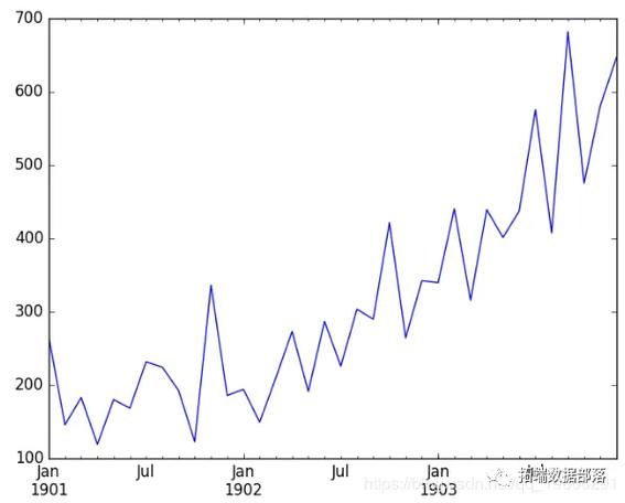
Observation: The plot clearly shows an upward trend and seasonality. The variance also increases over time. This is a classic non-stationary time series.

Step 2: Check for Stationarity and Determine d

We'll use the Augmented Dickey-Fuller (ADF) test. The null hypothesis is that the time series is non-stationary. If the p-value is less than a common threshold (e.g., 0.05), we reject the null hypothesis and conclude the series is stationary.

def adf_test(series):
    result = adfuller(series)
    print('ADF Statistic: %f' % result[0])
    print('p-value: %f' % result[1])
    print('Critical Values:')
    for key, value in result[4].items():
        print('\t%s: %.3f' % (key, value))
# ADF test on the original data
print("--- ADF Test on Original Data ---")
adf_test(df['Passengers'])
# The p-value is high (> 0.05), so we fail to reject the null hypothesis.
# The series is non-stationary. Let's difference it.
df_diff = df['Passengers'].diff().dropna()
# ADF test on the differenced data
print("\n--- ADF Test on Differenced Data (d=1) ---")
adf_test(df_diff)
# Plot the differenced data
plt.figure(figsize=(12, 6))
plt.plot(df_diff)'Differenced Airline Passengers (d=1)')
plt.xlabel('Date')
plt.ylabel('Differenced Passengers')
plt.grid(True)
plt.show()

Observation:

• Original Data: p-value is very high (e.g., 0.99), confirming non-stationarity.
• Differenced Data: The p-value is now very low (e.g., 0.05), so we can reject the null hypothesis. The series is now stationary. This suggests we should use d = 1.

Step 3: Identify p and q using ACF and PACF Plots

Now we plot the Autocorrelation Function (ACF) and Partial Autocorrelation Function (PACF) on our stationary data (df_diff).

• PACF(p): Helps identify the p value. Look for the lag where the PACF plot "cuts off" (drops sharply to zero).
• ACF(q): Helps identify the q value. Look for the lag where the ACF plot "cuts off".

fig, (ax1, ax2) = plt.subplots(2, 1, figsize=(12, 8))
# Plot PACF - helps determine 'p'
plot_pacf(df_diff, lags=14, ax=ax1)
ax1.set_title('Partial Autocorrelation Function (PACF)')
# Plot ACF - helps determine 'q'
plot_acf(df_diff, lags=14, ax=ax2)
ax2.set_title('Autocorrelation Function (ACF)')
plt.tight_layout()
plt.show()

Interpretation:

• PACF Plot: The PACF has a significant spike at lag 1 and then cuts off. This suggests p = 1.
• ACF Plot: The ACF has significant spikes at lags 1, 2, 3, and 10, 11, 12, etc. The seasonal part is strong, but for a simple ARIMA model, we look at the first few lags. The ACF tails off slowly, but a common starting point is to take the lag before it cuts off. Let's try q = 1.

So, our initial model is ARIMA(1, 1, 1).

Step 4: Fit the ARIMA Model

Now we fit the model using the parameters we identified.

# Fit the ARIMA model
model = ARIMA(df['Passengers'], order=(1, 1, 1))
model_fit = model.fit()
# Print the model summary
print(model_fit.summary())

The summary() output is very useful. It shows the coefficients, their statistical significance (P>|z|), and information criteria like AIC and BIC. A lower AIC/BIC is generally better.

Step 5: Check Model Residuals

A good model's residuals should be uncorrelated, like white noise. We can check this visually and with the Ljung-Box test.

# Get the residuals
residuals = model_fit.resid
# Plot residuals
plt.figure(figsize=(12, 6))
plt.plot(residuals)'Residuals of the ARIMA Model')
plt.axhline(0, color='red', linestyle='--')
plt.grid(True)
plt.show()
# Plot ACF of residuals
plot_acf(residuals, lags=14)'ACF of Residuals')
plt.show()
# Ljung-Box test on residuals
# The null hypothesis is that the residuals are independently distributed (no autocorrelation).
lb_test = acorr_ljungbox(residuals, lags=10, return_df=True)
print("\nLjung-Box Test on Residuals:")
print(lb_test)

Interpretation:

• Residual Plot: The residuals should look random with no obvious patterns. They seem to fluctuate around zero.
• ACF of Residuals: There should be no significant spikes. If there are, it means the model hasn't captured all the information in the data.
• Ljung-Box Test: If the p-values (lb_pvalue) are all greater than 0.05, we fail to reject the null hypothesis, meaning the residuals are likely white noise. This is what we want!

Step 6: Make Forecasts

Finally, let's use our model to forecast future values. We'll forecast the next 12 months and plot the results.

# Forecast the next 12 months
forecast_steps = 12
forecast = model_fit.forecast(steps=forecast_steps)
# Get the confidence intervals
forecast_ci = model_fit.get_forecast(steps=forecast_steps).conf_int()
# Create a new DataFrame for the forecast
forecast_index = pd.date_range(start=df.index[-1], periods=forecast_steps + 1, freq='MS')[1:]
forecast_df = pd.DataFrame({'Forecast': forecast}, index=forecast_index)
# Plot the results
plt.figure(figsize=(14, 7))
plt.plot(df['Passengers'], label='Observed')
plt.plot(forecast_df['Forecast'], color='red', label='Forecast')
plt.fill_between(forecast_index,
                 forecast_ci.iloc[:, 0],
                 forecast_ci.iloc[:, 1], color='pink', alpha=0.3, label='95% Confidence Interval')'Airline Passengers Forecast')
plt.xlabel('Date')
plt.ylabel('Number of Passengers')
plt.legend()
plt.grid(True)
plt.show()

Advanced Considerations: SARIMA

The standard ARIMA model does not handle seasonality well. For that, we use SARIMA (Seasonal ARIMA).

The SARIMA model has an additional set of parameters (P, D, Q, m) where:

• P, D, Q: The seasonal AR, I, and MA terms.
• m: The number of time steps for a single seasonal period (e.g., m=12 for monthly data with a yearly seasonality).

The full notation is SARIMA(p, d, q)(P, D, Q, m).

You can fit a SARIMA model in Python using statsmodels:

from statsmodels.tsa.statespace.sarimax import SARIMAX
# Define the SARIMA model
# (1, 1, 1) for the non-seasonal part
# (1, 1, 1, 12) for the seasonal part (P, D, Q, m)
sarima_model = SARIMAX(df['Passengers'], 
                       order=(1, 1, 1), 
                       seasonal_order=(1, 1, 1, 12))
# Fit the model
sarima_fit = sarima_model.fit(disp=False)
# Print summary
print(sarima_fit.summary())
# Forecast with SARIMA
sarima_forecast = sarima_fit.get_forecast(steps=12)
sarima_forecast_df = sarima_forecast.predicted_mean
sarima_ci = sarima_forecast.conf_int()
# Plot SARIMA results
plt.figure(figsize=(14, 7))
plt.plot(df['Passengers'], label='Observed')
plt.plot(sarima_forecast_df, color='green', label='SARIMA Forecast')
plt.fill_between(sarima_forecast_df.index,
                 sarima_ci.iloc[:, 0],
                 sarima_ci.iloc[:, 1], color='lightgreen', alpha=0.3, label='95% CI')'SARIMA Forecast for Airline Passengers')
plt.legend()
plt.grid(True)
plt.show()

Notice how the SARIMA model's forecast captures the seasonal pattern much more effectively than the simple ARIMA model.

How to Automatically Find the Best Parameters (p, d, q)

Manually identifying p, d, and q can be tedious. You can automate this process by iterating through different combinations and selecting the model with the lowest AIC.

import itertools
import warnings
# Define the p, d, and q parameters to take any value between 0 and 2
p = d = q = range(0, 3)
# Generate all different combinations of p, d, and q triplets
pdq = list(itertools.product(p, d, q))
# Generate all different combinations of seasonal p, d, q and m
seasonal_pdq = [(x[0], x[1], x[2], 12) for x in list(itertools.product(p, d, q))]
warnings.filterwarnings("ignore") # specify to ignore warning messages
best_aic = np.inf
best_pdq = None
best_seasonal_pdq = None
best_model = None
for param in pdq:
    for param_seasonal in seasonal_pdq:
        try:
            mod = SARIMAX(df['Passengers'],
                          order=param,
                          seasonal_order=param_seasonal,
                          enforce_stationarity=False,
                          enforce_invertibility=False)
            results = mod.fit()
            print(f'SARIMA{param}x{param_seasonal} - AIC:{results.aic:.2f}')
            # Find the best model
            if results.aic < best_aic:
                best_aic = results.aic
                best_pdq = param
                best_seasonal_pdq = param_seasonal
                best_model = results
        except Exception as e:
            print(f"Unexpected error: {e}")
            continue
print(f'\nBest SARIMA{best_pdq}x{best_seasonal_pdq} - AIC:{best_aic:.2f}')

This grid search will help you find the optimal parameters for your SARIMA model.