Of course! The terms "row" and "column" are fundamental when working with data in Python, especially in libraries like NumPy and Pandas. They refer to the two dimensions of a two-dimensional data structure, like a table or a matrix.

Let's break it down with clear analogies and code examples.
The Core Concept: A Grid Analogy
Imagine a spreadsheet or a grid.
- A Row is a horizontal line of data. It goes from left to right.
- A Column is a vertical line of data. It goes from top to bottom.
| Column 0 | Column 1 | Column 2 |
|---|---|---|
| Row 0 | A0 | B0 |
| Row 1 | A1 | B1 |
| Row 2 | A2 | B2 |
In programming, we typically use zero-based indexing, meaning we start counting from 0.
Working with Rows and Columns in Python Lists
Python's built-in list is the most basic way to represent a table. You create a table by having a list of lists (a list where each element is another list).
- The outer list contains the rows.
- Each inner list represents a single row.
To access a specific element, you use two indices: my_table[row_index][column_index].
# A simple table represented as a list of lists
# Each inner list is a row.
data = [
    ["Alice", 28, "Engineer"],  # Row 0
    ["Bob",   34, "Designer"],  # Row 1
    ["Charlie", 29, "Manager"]  # Row 2
]
# --- Accessing Elements ---
# Get an entire row (e.g., the data for Bob)
row_1 = data[1]
print(f"Entire Row 1: {row_1}")
# Output: Entire Row 1: ['Bob', 34, 'Designer']
# Get a specific element (e.g., Bob's age)
# It's at Row 1, Column 1
bobs_age = data[1][1]
print(f"Bob's Age: {bobs_age}")
# Output: Bob's Age: 34
# Get an entire column (e.g., all names)
# This requires iterating through each row and picking the 0th element
column_0_names = [row[0] for row in data]
print(f"All Names (Column 0): {column_0_names}")
# Output: All Names (Column 0): ['Alice', 'Bob', 'Charlie']
Key Takeaway for Lists:
data[row]gets you a whole row.data[row][col]gets you a single cell.- Getting a column requires looping through all the rows.
Working with Rows and Columns in NumPy
NumPy is the fundamental package for scientific computing in Python. Its ndarray (N-dimensional array) object is highly optimized for numerical operations.
- The first axis (axis=0) corresponds to rows.
- The second axis (axis=1) corresponds to columns.
NumPy provides powerful and intuitive syntax for slicing rows and columns.
import numpy as np
# Create a NumPy array from our list data
data_np = np.array([
    ["Alice", 28, "Engineer"],
    ["Bob",   34, "Designer"],
    ["Charlie", 29, "Manager"]
])
print("Original NumPy Array:")
print(data_np)
print("-" * 20)
# --- Accessing Rows ---
# Get a single row (returns a 1D array)
row_1_np = data_np[1]
print(f"Entire Row 1: {row_1_np}")
# Output: Entire Row 1: ['Bob' '34' 'Designer']
# Get multiple rows using slicing (returns a 2D array)
rows_0_and_1 = data_np[0:2]
print(f"Rows 0 and 1:\n{rows_0_and_1}")
# Output:
# Rows 0 and 1:
# [['Alice' '28' 'Engineer']
#  ['Bob' '34' 'Designer']]
print("-" * 20)
# --- Accessing Columns ---
# This is where NumPy shines!
# To get a column, you use a colon `:` for the row index and the column index.
# The colon `:` means "select all rows".
# Get a single column (returns a 1D array)
column_1_ages = data_np[:, 1]
print(f"All Ages (Column 1): {column_1_ages}")
# Output: All Ages (Column 1): ['28' '34' '29']
# Get multiple columns using slicing
names_and_titles = data_np[:, 0:2]
print(f"Names and Titles (Columns 0 & 1):\n{names_and_titles}")
# Output:
# Names and Titles (Columns 0 & 1):
# [['Alice' '28']
#  ['Bob' '34']
#  ['Charlie' '29']]
Key Takeaway for NumPy:
data[row]ordata[row, :]gets you a row.data[:, col]gets you a column.- The is the key to selecting all elements along an axis.
Working with Rows and Columns in Pandas
Pandas is built on top of NumPy and is the go-to library for data analysis and manipulation. Its primary data structure is the DataFrame, which is essentially a labeled 2D table.
- Rows are identified by an index (can be numbers or labels).
- Columns are identified by column names.
This makes Pandas the most intuitive for working with real-world tabular data.
import pandas as pd
# Create a Pandas DataFrame
df = pd.DataFrame(data, columns=["Name", "Age", "Title"])
print("Original Pandas DataFrame:")
print(df)
print("-" * 30)
# --- Accessing Rows ---
# Get a row by its integer index (using .iloc[])
# iloc stands for "integer location"
row_1_df = df.iloc[1]
print(f"Row 1 using .iloc[]:\n{row_1_df}")
# Output:
# Row 1 using .iloc[]:
# Name Bob
# Age 34 Designer
# Name: 1, dtype: object
# Get a row by its label (using .loc[])
# Let's set the index to be the names
df_indexed = df.set_index("Name")
row_bob = df_indexed.loc["Bob"]
print(f"Row for 'Bob' using .loc[]:\n{row_bob}")
# Output:
# Row for 'Bob' using .loc[]:
# Age 34 Designer
# Name: Bob, dtype: object
print("-" * 30)
# --- Accessing Columns ---
# This is extremely simple in Pandas!
# Just use the column name in square brackets.
# Get a single column (returns a Pandas Series)
column_1_ages_df = df["Age"]
print(f"All Ages (Column 'Age'):\n{column_1_ages_df}")
# Output:
# All Ages (Column 'Age'):
# 0 28
# 1 34
# 2 29
# Name: Age, dtype: int64
# Get multiple columns by passing a list of names
names_and_titles_df = df[["Name", "Title"]]
print(f"Names and Titles (multiple columns):\n{names_and_titles_df}")
# Output:
# Names and Titles (multiple columns):
# Name Title
# 0 Alice Engineer
# 1 Bob Designer
# 2 Charlie Manager
Key Takeaway for Pandas:
- Rows: Use
.iloc[]for integer-location-based indexing and.loc[]for label-based indexing. - Columns: Use
df["ColumnName"]ordf[["Col1", "Col2"]].
Summary Table
| Library/Structure | How to Access a Row | How to Access a Column | Best For |
|---|---|---|---|
| Python List | data[row_index] |
[row[col_index] for row in data] |
Simple, non-tabular data. |
| NumPy Array | data[row_index] or data[row_index, :] |
data[:, col_index] or data[:, col_start:col_end] |
Numerical computations, matrix math. |
| Pandas DataFrame | .iloc[row_index] or .loc[row_label] |
df["col_name"] or df[["col1", "col2"]] |
Data analysis, cleaning, and manipulation with labeled data. |